PTfS22: Assignment 11 (last): Halo exchange, networks, ray tracer reloaded (due July 25 11:59 a.m.)

Opened: Wednesday, 13 July 2022, 12:00 AM

Due: Monday, 25 July 2022, 12:00 PM

Note: A factor of 1.4 will be applied to the max credits for this assignment (for an overall credit of 140). This is the last assignment.

Halo exchange. Assume you have a parallel computer with a memory bandwidth of 80 GB/sec per node, an inter-node communication latency of 2 $ \mu s $, an asymptotic inter-node communication bandwidth of 3 Gbyte/s (full-duplex, per direction), and an (assumed) fully nonblocking fat-tree network. On this system we execute a double-precision 3D Jacobi smoother (as discussed in the lecture) with halo exchange. The per-node subdomain has $ N_d^3 $ elements. Assume that "perfect" spatial blocking is in place, i.e., the minimum code balance applies, and that intra-node parallelization is overhead free. You can also assume that the entire communication overhead is in the network communication (no time needed for buffer copying etc.). One halo layer must be communicated per subdomain face and direction (cubic domain decomposition).

(a) (5 crd) Calculate the maximum per-node memory-bound performance in LUP/s.
(b) (5 crd) Calculate the inter-node communication message length $ n_{1/2} $ in bytes at which half of the asymptotic effective communication bandwidth is attained.
(c) (10 crd) Calculate the linear subdomain size $ N_d $ where the communication to neighboring nodes becomes bandwidth bound. You may use the threshold from (b) as the criterion for "bandwidth bound."
(d) (10 crd) Calculate the linear subdomain size $ N_d $ where the update sweep takes the same amount of time as the communication of the halos to/from the six neighboring nodes. What do you conclude from the result? Can this "performance model" be correct?
Oversubscribed fat tree. (10 credits) Construct the largest possible fat-tree network with one leaf and one spine level out of 36-port QDR-InifinBand switches and 2:1 oversubscription. How many compute nodes can be connected to this hierarchy, and how many 36-port switches are needed?
Performance measurement. Use likwid-perfctr and its marker API to measure properties of the loop nest in the calc_tile() function in the ray tracer program (problem size 10000x10000). Start with the code in ~ptfs100h/GettingStarted/ray_omp.c (which already has OpenMP parallelization) and set the clock speed to 2.0 GHz.
Note that you can use command line arguments to set the image size and the tile size. To set an image size of 10000x10000 and a tile size of 1000x1000, use:
```
$ ./a.out 10000 1000
```
(a) (10 crd) Run the code with one thread. What is the double-precision FLOP rate per cycle?
(b) (10 crd) Determine if the floating-point instructions are of the SIMD type. I.e., is the code vectorized?
(c) (10 crd) Now run with 72 cores and static loop scheduling to measure the load imbalance in terms of flops across threads for a tile size of 500x500 pixels. What is the ratio of floating-point work between the core with the "heaviest" and the core with the "lightest" load? Hint: The parallel loop over the tiles uses a "runtime" schedule, i.e., you can use the OMP_SCHEDULE environment variable to set the loop schedule from the outside:
```
$ OMP_SCHEDULE=static likwid-perfctr ...blabla... ./a.out 10000 500
```
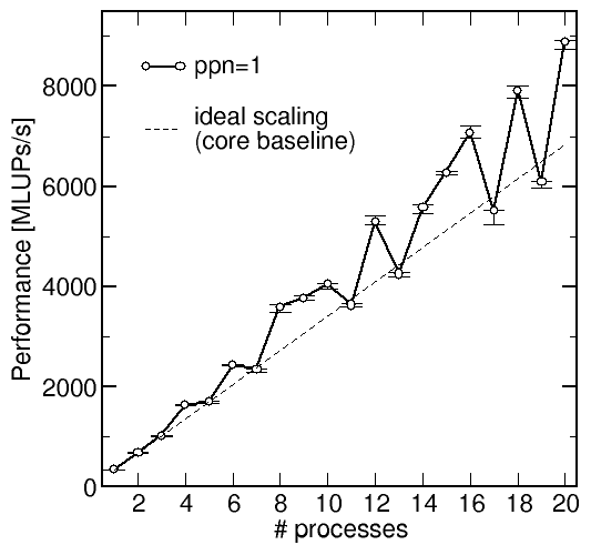Strong scaling of a 3D Jacobi solver. The image on the right shows strong scaling data for an MPI-parallel 3D Jacobi solver with Cartesian domain decomposition on the "Meggie" cluster at RRZE, running 1 MPI process per node on a fully nonblocking fat-tree (Omni-Path) network. The problem size was 1000³ grid points for an overall working set of 16 GB. Per node, Meggie has two CPUs of type "Xeon E5-2630 v4" with a memory bandwidth of 54 GB/s per socket and an L3 cache of 25 MiB. For the experiment, the clock frequency was fixed to 2.2 GHz.
The "whiskers" at each data point show the observed performance fluctuations across ten sweeps, so the erratic performance behavior cannot come from run-to-run variations. The dashed line shows theoretical (ideal) scaling with respect to the single-process baseline.
Note that the 3D domain decomposition is done in an "ideal" way: Subdomains are as cubic as possible according to the prime factors in the number of processes. The outer (z) dimension is always cut first, then the middle dimension, and then the inner dimension. Example: With 20 processes, we have a decomposition of $ n_x\times n_y\times n_z=2\times 2\times 5$, whereas at 10 processes we have $ n_x\times n_y\times n_z=1\times 2\times 5$.

(a) Where (i.e., at which numbers of processes) is the performance especially bad? Can communication overhead be the reason for this? How? (Or why not?) (5 crd)
(b) Looking at the ideal scaling line, we must conclude that some process numbers are better than others. In fact, superlinear scaling can be observed if we ignore the "bad" points. Superlinear scaling means that the performance with $N$ workers is larger than $N$ times the performance with one worker. Explain the reason for the superlinear scaling. (15 crd)
(c) Assuming that the code is memory bound, calculate the expected performance ratio between a "good" measurement (e.g., the one at 20 processes) and the ideal scaling line. Why does the measurement not match the model? (10 crd)